How to Calculate NPV (Net Present Value) in Excel
NPV is an acronym for Net Present Value. It's a financial metric used to evaluate a project's likelihood of giving good or bad return in future. NPV can be simply stated as the difference between present value of cash inflows and present value of cash outflows. A positive NPV value indicates that the project is likely to yield profit in future, while a negative NPV value forecasts a bad return.
NPV can be easily calculated with our NPV Calculator, but that works only if you have an internet connection. For offline use, spreadsheet programs like Excel, LibreOffice Calc, OpenOffice Calc, etc. are still good choices. Let's find out how to calculate NPV in Excel.
NPV Formula in Excel
Formula for calculating NPV in Excel is a little tricky. Excel's default function is NPV(RATE, value1, value2, ...). The result that you get with this formula doesn't match the actual value because the initial investment (or the investment made at the start of the project) is also taken into account as the first cash-flow value. That's why the correct formula for Excel should be:
NPV(RATE, value1, value2, ...) − Initial Investment
NPV Calculation in Excel with Example
Let's find out how we can use the above suggested formula for calculating NPV in Excel. Before anything we must have all the values ready to fill. As an example, let's consider the table below. Data already given in this table are initial investment, rate and cash-flows for each year starting from Year 1 to Year 5.
| Discount Rate | 8.50% |
| Initial Investment | 1200 |
| Year 1 | 120 |
| Year 2 | 110 |
| Year 3 | -100 |
| Year 4 | 200 |
| Year 5 | -50 |
Step 1: Fill the values in Excel
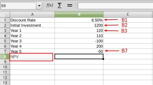
You can choose any column and start with any row in Excel. In this example, we will use Column "A" for labels and Column "B" for its values (refer to the picture given below). For instance, row 1 of Column "A" is labeled as "Discount Rate" with row 1 of Column "B" as its value. Therefore A1 is "Discount Rate" and B1 is "8.50%". Similarly, we will fill all the remaining data into the spreadsheet. A2 cell is the "Initial Investment" and B2 cell is "1200". "Year 1" starts with A3 cell followed by other years below it. The cash-flows value in each year starts with B3 cell and goes all the way to B7 cell. The final value of NPV is going to be written in B8 cell.
Step 2: Applying the function or formula
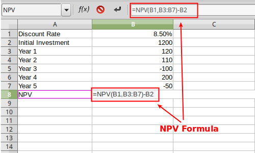
Next, select the corresponding column to NPV which is B8 cell and type the NPV formula as suggested above to calculate the NPV value inside it. In the B8 cell type "=NPV(B1,B3:B7)-B2". As you do this, the input field for Function will get the same value as exactly shown in the picture below. Note that, "B3:B7" is the short form of "B3,B4,B5,B6,B7" and it means the same.
Step 3: Getting the NPV result
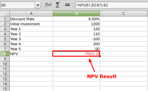
Finally, after typing the above function into the B8 cell or function input (fx) area of Excel, hit the "Enter" key. This will reflect the calculated NPV value inside the same cell (B8). In this case, the NPV would be -963.19, which is rounded off to two decimal places. The negative NPV result indicates that the project or investment is likely to make a loss in the future.
That's it. This is how to calculate NPV in an Excel spreadsheet correctly.
Read more: How to calculate CAGR in Excel